Ever since matplotlib’s basemap has been deprecated I wanted to take a closer look at the cartopy project so that I can keep using python for displaying data on maps. Fortunately, this week’s #tidytuesday project concerns spatially explicit data of African water sources provided by Water Point Data Exchange.

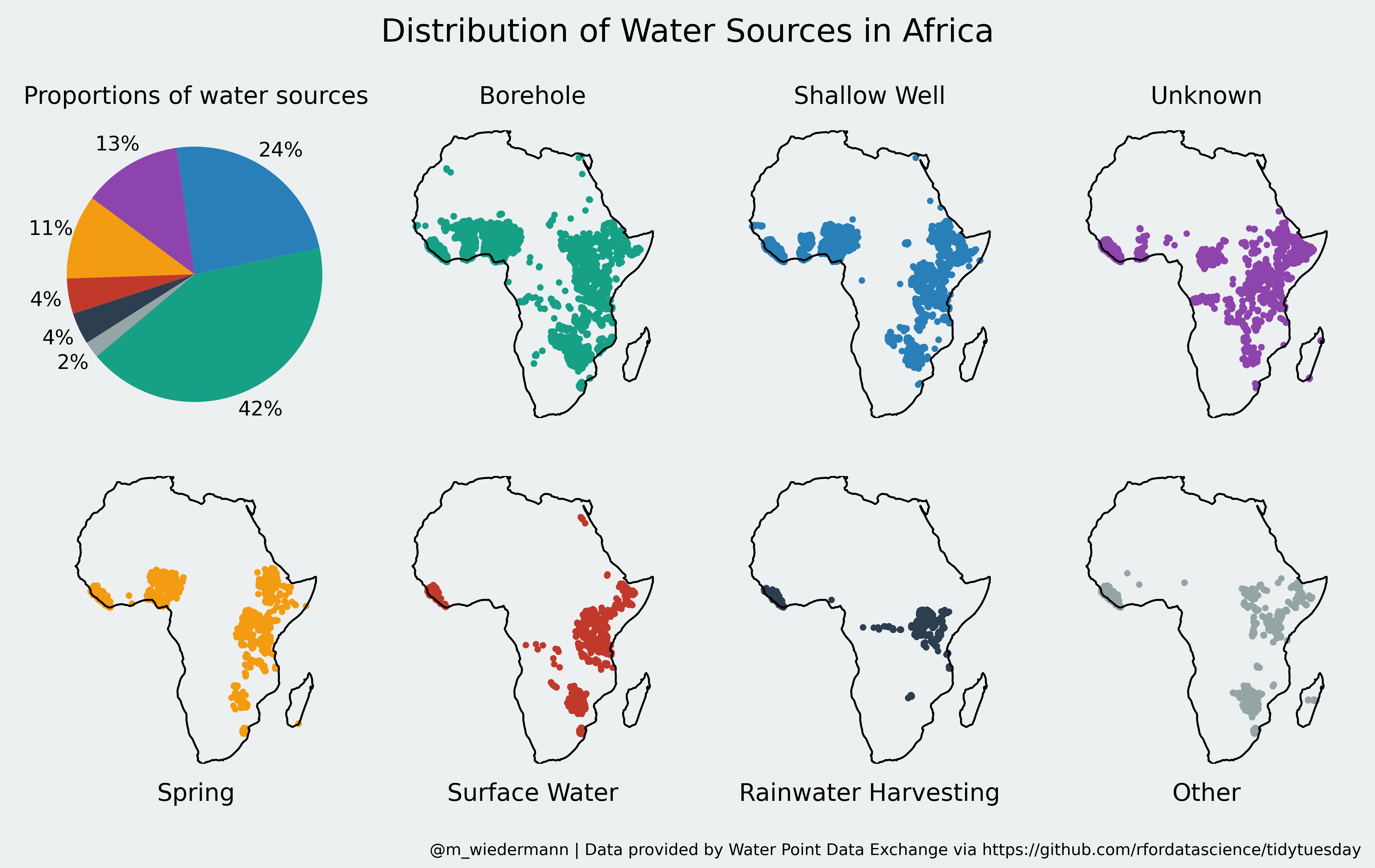
The data is provided as a csv table which, among others, contains the longitudinal and latitudinal position of a water source as well as its type (e.g., a spring, a borehole or a well). An interesting visualization task is to display the different types on a map to find out which regions rely on specific types for their water supply.

Upon first inspection I found that the data contains some points that are falsely assigned to a location outside Africa (some coordinates for instance fall into Antarctica). Since the purpose of this post is to illustrate the functionality of cartopy (and shapely) I won’t dig into why this problem arises, but simply ignore all invalid data points. However, this means that there is some preprocessing to do. Specifically we will:

1. Download the data using requests
2. Load the data into a pandas dataframe
3. Use cartopy.io.shapereader to obtain shapefiles of all African countries
4. Use geopandas to construct a single shapefile corresponding to the boundary of the African continent as the union of all country-shapefiles
5. Remove all data points which do not fall into our obtained shapefile
6. Put the types of water sources into a reduced number of meaningful categories
7. Plot all locations of each unique type of water source on a different map

Before going into the specifics of the code, here is the final version of the infographic. I decided against showing country borders to keep the whole graphic simple and concise:

Let’s quickly go through the code that is needed to obtain the above figure. You can also get the entire source code in a single jupyter notebook from my github.

We start with the necessary imports. Specifically, we need pandas to load and manipulate the data, shapely and geopandas to obtain a shapefile for Africa and cartopy for drawing the map of Africa based on our obtained shapefile.

import pandas as pd
from shapely.geometry import Point
from shapely.ops import cascaded_union
from matplotlib import pyplot as plt
from cartopy import crs as ccrs
from cartopy import feature as cfeature
import cartopy.io.shapereader as shpreader
import geopandas as gpd
import requests
import os

We then need some global variables. The different COLORS will be used to indicate the different types of water source. Here, we use the default palette from flatuicolors.com. We also need to specify the url for the downloading the input data from tidytuesday’s github:

COLORS = ["#16a085", "#2980b9", "#8e44ad", "#f39c12", "#c0392b", "#2c3e50", "#95a5a6"]
URL = "https://raw.githubusercontent.com/rfordatascience/tidytuesday/master/data/2021/2021-05-04/water.csv"

Next, we need some functions for achieving the tasks outlined above: download_data obtains the raw input data from the url specified above, load_data reads the data into a pandas dataframe, shapefile_continent creates a single shapefile that corresponds to the boundaries of a given continent and filter_data removes all data points that fall outside of this shapefile. Ultimately, harmonize_water_sources aggregates the types of water sources such that for instance all springs (Protected Spring, Unprotected Spring, Undefined Spring) are simply labelled as Spring:

def download_data(url, target="water.csv"):
    """Download input file from the web."""
    if not os.path.exists(target):
        r = requests.get(url, allow_redirects=True)
        open(target, 'wb').write(r.content)

def load_data(infile="water.csv"):
  return pd.read_csv(infile)

def shapefile_continent(continent="Africa"):
    """Get a single combined shapefile for a specified continent."""
    shpfilename = shpreader.natural_earth(resolution='110m', category='cultural', name='admin_0_countries')
    reader = shpreader.Reader(shpfilename)
    valid_shapes = [record.geometry for record in reader.records() if record.attributes["CONTINENT"] == continent]

    return gpd.GeoSeries(cascaded_union(valid_shapes))

def filter_data(data, continent="Africa"):
    """Remove all data points that are not within the specified continent."""
    shapefile = shapefile_continent(continent=continent)
    mask = [shapefile.contains(Point(lon, lat)).bool() for lat, lon in zip(data["lat_deg"], data["lon_deg"])]
    return data[mask]

def harmonize_water_sources(data):
    """Replace water_source by more general attributes"""

    # Summarize all sources that appear only in few instances as others
    count = data.groupby("water_source").count()["row_id"]
    others = count[count < 0.01 * len(data)].index.tolist()

    data["water_source"] = data['water_source'].replace(others,'Other')
    data["water_source"] = data['water_source'].replace(['Protected Spring', 'Unprotected Spring', 'Undefined Spring'],'Spring')
    data["water_source"] = data['water_source'].replace(['Protected Shallow Well', 'Unprotected Shallow Well', 'Undefined Shallow Well'],'Shallow Well')
    data["water_source"] = data['water_source'].replace(['Surface Water (River/Stream/Lake/Pond/Dam)'],'Surface Water')
    data.water_source = data.water_source.fillna("Unknown")

    return data

We can now run the above functions in order. I suggest to do this in a separate block of code since harmonize_water_sources takes a minute or so to complete:

# Load the data, filter out all points outside Africa and categorize the water sources
download_data(url=URL)
data = load_data()
data = filter_data(data)
data = harmonize_water_sources(data)

Finally, we can visualize our preprocessed data. We start with a pie chart that displays the proportions of each type of water source. The colors correspond to the different water sources that are displayed on the maps. Each map is drawn on its own axis, since due to the large density of data points we would not be able to tell any differences in the spatial distribution of water sources if we were to show them all in a single map. Ultimately, we finalize the figure by doing some adjustments to the axis-positions and setting a title as well as some meta-info:

fig = plt.figure(figsize=(9.5, 6))

# Get the shapefile for Africa
shpfile = shapefile_continent(continent="Africa")

# Start by drawing a pie chart for the proportions of each water source
ax = fig.add_subplot(2,4,1, projection=ccrs.Robinson())
sources_count = data.groupby("water_source").count()["row_id"].sort_values(ascending=False)
cs = sources_count.plot.pie(colors=COLORS, ax=ax, labels=None, ylabel="", autopct='%1.0f%%', pctdistance=1.18, startangle=220)
ax.axis('equal')
ax.set_title("Proportions of water sources", y=1.05)

# Iterate over each source and draw its locations in unique color on separate maps
for i, (color, source) in enumerate(zip(COLORS, sources_count.index.to_list())):

    ax = fig.add_subplot(2,4,i+2, projection=ccrs.Robinson())
    ax.set_extent([-21, 60, -40, 40], crs=ccrs.PlateCarree())

    x0, y0, x1, y1 = shpfile.bounds.loc[0].values
    ax.set_extent([x0, x1, y0, y1], crs=ccrs.PlateCarree())
    ax.add_geometries(shpfile, crs=ccrs.PlateCarree(), facecolor="None")
    ax.axis('off')

    x = data[data.water_source == source].lon_deg
    y = data[data.water_source == source].lat_deg
    ax.scatter(x=x, y=y, c=color, s=5, transform=ccrs.PlateCarree(), rasterized=True)

    ax.set_title(source, y=1.05 if i < 3 else -0.17)

# Finalize the figure
plt.subplots_adjust(wspace=0.0, hspace=0.2, left=0.02, right=1, top=0.85, bottom=0.12)
fig.patch.set_facecolor('#ecf0f1')
plt.suptitle("Distribution of Water Sources in Africa", fontsize=16)
fig.text(0.99, 0.015, "@m_wiedermann | Data provided by Water Point Data Exchange via https://github.com/rfordatascience/tidytuesday", ha="right", size=8)
plt.savefig("water_sources.jpg", dpi=500)
plt.show()

That’s it. For reproducing the figure you can either copy all the above snippets into a single file or jupyter notebook and run the code on your local machine. Alternatively you can get the entire code in a single jupyter notebook from my github.

As a final remark, note that there are a lot of issues that need to be taken care of if we were to draw any conclusions from this data set. There seems to be quite some heterogeneity in the spatial distribution of water sources which might point towards incomplete or low quality data over certain regions. We also did not dig any deeper into why some coordinates are located outside of Africa even though the corresponding water source allegedly belongs to an African country. As such, the purpose of this post is merely to showcase some potential applications of cartopy and shapely without worrying too much about data quality and implications.

Back to posts